Creating Images

This example focuses on creating 2D image objects in Sigima.

There are three primary methods to create images in Sigima:

1. Synthetic data generation: Using built-in parameter classes to create standard

   image types (Gaussian, ramp, random distributions, etc.)

2. Loading from files: Importing data from various file formats

3. From NumPy arrays: Creating objects directly from existing arrays

Each method has its use cases, and Sigima provides a consistent interface for working with data regardless of its origin.

For visualization, we use helper functions from the sigima.viz module. This allows us to focus on Sigima’s functionality rather than visualization details.

Importing necessary modules

First of all, we need to import the required modules.

import numpy as np

import sigima
from sigima import viz
from sigima.tests import helpers

Method 1: Creating images from synthetic parameters

Similar to signals, Sigima can generate synthetic images using parameter classes.

Available image types include:

• Distributions: Normal (Gaussian noise), Uniform, Poisson

• Analytical functions: 2D Gaussian, 2D ramp (bilinear form)

• Blank images: Zeros

# Create a 2D Gaussian image
gaussian_param = sigima.create_image_parameters(
    sigima.ImageTypes.GAUSS,
    title="Synthetic 2D Gaussian",
    height=300,
    width=300,
    xlabel="X Position",
    ylabel="Y Position",
    zlabel="Intensity",
    xunit="µm",
    yunit="µm",
    zunit="counts",
    x0=0.0,  # Center x position
    y0=0.0,  # Center y position
    sigma=1.5,  # Width
    a=1000.0,  # Amplitude
)

gaussian_img = sigima.create_image_from_param(gaussian_param)

# Create a ramp image (gradient)
ramp_param = sigima.create_image_parameters(
    sigima.ImageTypes.RAMP,
    title="Synthetic 2D Ramp",
    height=200,
    width=200,
    xlabel="X Position",
    ylabel="Y Position",
    zlabel="Value",
    xunit="mm",
    yunit="mm",
    zunit="a.u.",
    x0=-5.0,
    y0=-5.0,
    a=0.5,  # X slope
    b=0.3,  # Y slope
)

ramp_img = sigima.create_image_from_param(ramp_param)

print("\n✓ Synthetic images created")
print(f"  - {gaussian_img.title}: {gaussian_img.data.shape}")
print(f"  - {ramp_img.title}: {ramp_img.data.shape}")

# Visualize synthetic images
viz.view_images_side_by_side([gaussian_img, ramp_img], title="Synthetic Images")

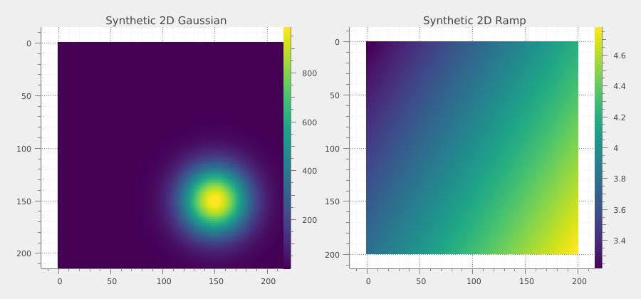
✓ Synthetic images created
  - Synthetic 2D Gaussian: (300, 300)
  - Synthetic 2D Ramp: (200, 200)

Method 2: Loading images from files

Sigima supports a wide range of image file formats, both common and scientific.

Supported formats include:

• Common formats: BMP, JPEG, PNG, TIFF, JPEG 2000

• Scientific formats: DICOM, Andor SIF, Spiricon, Dürr NDT

• Data formats: NumPy (.npy), MATLAB (.mat), HDF5 (.h5img)

• Text formats: CSV, TXT, ASC (with coordinate support)

# Load an image from a JPEG file
filename = helpers.get_test_fnames("fiber.jpg")[0]
img_jpeg = sigima.read_image(filename)
img_jpeg.title = "Fiber Image (from JPEG)"

# Load an image from a NumPy file
filename = helpers.get_test_fnames("flower.npy")[0]
img_npy = sigima.read_image(filename)
img_npy.title = "Test Image (from NumPy)"

print("\n✓ Images loaded from files")
print(f"  - {img_jpeg.title}: {img_jpeg.data.shape}")
print(f"  - {img_npy.title}: {img_npy.data.shape}")

# Visualize images loaded from files
viz.view_images_side_by_side([img_jpeg, img_npy], title="Images from Files")

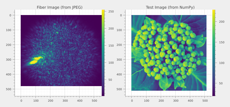
✓ Images loaded from files
  - Fiber Image (from JPEG): (480, 640)
  - Test Image (from NumPy): (512, 512)

Method 3: Creating images from NumPy arrays

Convert existing NumPy arrays into Sigima image objects to add metadata, coordinate systems, and enable advanced processing.

# Create a synthetic pattern: interference fringes
size = 256
x = np.linspace(-10, 10, size)
y = np.linspace(-10, 10, size)
X, Y = np.meshgrid(x, y)

# Interference pattern
pattern = np.cos(2 * np.pi * X / 3) * np.cos(2 * np.pi * Y / 3)
pattern = ((pattern + 1) / 2 * 255).astype(np.uint8)

img_interf = sigima.create_image(
    title="Interference Pattern (from array)",
    data=pattern,
    units=("mm", "mm", "intensity"),
    labels=("X", "Y", "Signal"),
)

# Create another image: radial gradient with noise
radial = np.exp(-(X**2 + Y**2) / 20)
rng = np.random.default_rng(123)
radial = radial + rng.normal(0, 0.05, radial.shape)
radial = np.clip(radial, 0, 1)

img_radial = sigima.create_image(
    title="Radial Gradient (from array)",
    data=radial.astype(np.float32),
    units=("µm", "µm", "a.u."),
    labels=("X", "Y", "Amplitude"),
)

print("\n✓ Images created from NumPy arrays")
print(f"  - {img_interf.title}: {img_interf.data.shape}")
print(f"  - {img_radial.title}: {img_radial.data.shape}")

# Visualize images created from NumPy arrays
viz.view_images_side_by_side([img_interf, img_radial], title="Images from Arrays")

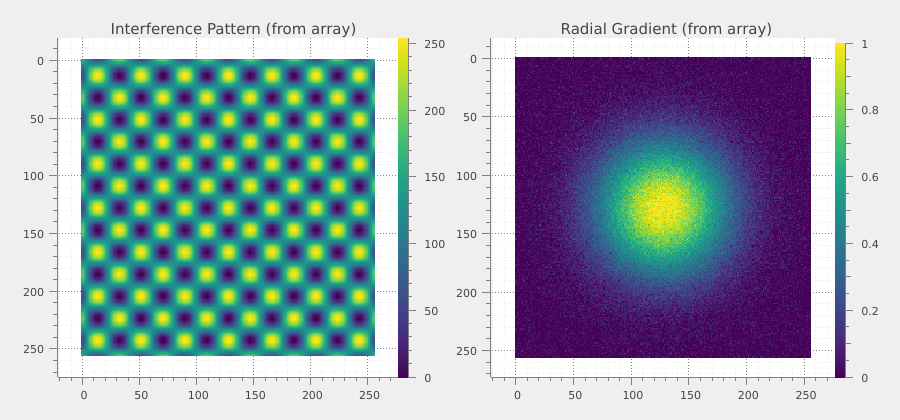
✓ Images created from NumPy arrays
  - Interference Pattern (from array): (256, 256)
  - Radial Gradient (from array): (256, 256)

Summary

This example demonstrated the three main ways to create images in Sigima:

1. Synthetic generation: Fast creation of standard mathematical functions and distributions using parameter classes. Perfect for testing and simulation.

2. File loading: Read data from various scientific and common file formats, with automatic format detection and metadata extraction. Essential for working with experimental data.

3. NumPy array conversion: Wrap existing array data with Sigima’s rich metadata and processing capabilities. Ideal for custom workflows and integration with other Python libraries.

All three methods produce equivalent Sigima objects that can be processed, analyzed, and visualized using the same set of tools and functions. Choose the method that best fits your workflow and data source.