
Note
Go to the end to download the full example code.
Creating Signals#
This example focuses on creating 1D signal objects in Sigima.
There are three primary methods to create signals in Sigima:
- Synthetic data generation: Using built-in parameter classes to create standard
signal types (Gaussian, sine waves, random distributions, etc.)
Loading from files: Importing data from various file formats
From NumPy arrays: Creating objects directly from existing arrays
Each method has its use cases, and Sigima provides a consistent interface for working with data regardless of its origin.
For visualization, we use helper functions from the sigima.viz module.
This allows us to focus on Sigima’s functionality rather than visualization details.
Importing necessary modules#
First of all, we need to import the required modules.
from pprint import pprint  # For pretty-printing metadata

import numpy as np

import sigima
from sigima import viz
from sigima.tests import helpers
Method 1: Creating signals from synthetic parameters#
Sigima provides built-in generators for common signal types. This is the most convenient method when you need standard mathematical functions or random distributions.
Available signal types include:
Mathematical functions: Gaussian, Lorentzian, Sinc, Sine, Cosine, etc.
Random distributions: Normal, Uniform, Poisson
Standard waveforms: Square, Sawtooth, Triangle
Special functions: Planck (blackbody), Linear chirp, Step, Exponential
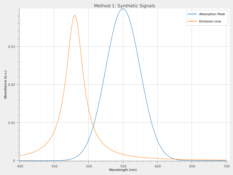
# Let's consider a spectroscopy context, where we often deal with Gaussian and
# Lorentzian peaks representing absorption and emission lines.
#
# Create a Gaussian signal: this represents an absorption peak in spectroscopy.
gaussian_param = sigima.create_signal_parameters(
    sigima.SignalTypes.GAUSS,  # Type of signal to create
    title="Absorption Peak",
    size=500,  # Number of points
    xlabel="Wavelength",
    ylabel="Absorbance",
    xunit="nm",
    yunit="a.u.",
    xmin=400.0,  # Minimum x value (wavelength)
    xmax=700.0,  # Maximum x value
    a=2.5,  # Amplitude
    mu=550.0,  # Center wavelength (green light)
    sigma=25.0,  # Peak width
)
signal_synthetic = sigima.create_signal_from_param(gaussian_param)

# Create a Lorentzian signal representing a different spectral line: this represents an
# emission line in atomic emission spectroscopy.
lorentzian_param = sigima.create_signal_parameters(
    sigima.SignalTypes.LORENTZ,
    title="Emission Line",
    size=500,
    xlabel="Wavelength",
    ylabel="Intensity",
    xunit="nm",
    yunit="a.u.",
    xmin=400.0,
    xmax=700.0,
    a=1.8,  # Amplitude
    mu=480.0,  # Center wavelength (blue light)
    sigma=15.0,  # Peak width
)
signal_lorentzian = sigima.create_signal_from_param(lorentzian_param)

print("✓ Synthetic signals created")
print(f"  - {signal_synthetic.title}: {signal_synthetic.y.shape[0]} points")
print(f"  - {signal_lorentzian.title}: {signal_lorentzian.y.shape[0]} points")

# Visualize synthetic signals
viz.view_curves(
    [signal_synthetic, signal_lorentzian], title="Method 1: Synthetic Signals"
)
✓ Synthetic signals created
  - Absorption Peak: 500 points
  - Emission Line: 500 points
Method 2: Loading signals from files#
Sigima can read signals from various file formats, automatically detecting the format and extracting metadata when available.
Supported formats include:
Text files: CSV, TXT (with automatic delimiter detection)
Scientific formats: HDF5 (.h5sig), MAT-Files (.mat), NumPy (.npy)
Specialized: MCA spectrum files (.mca), FT-Lab (.sig)
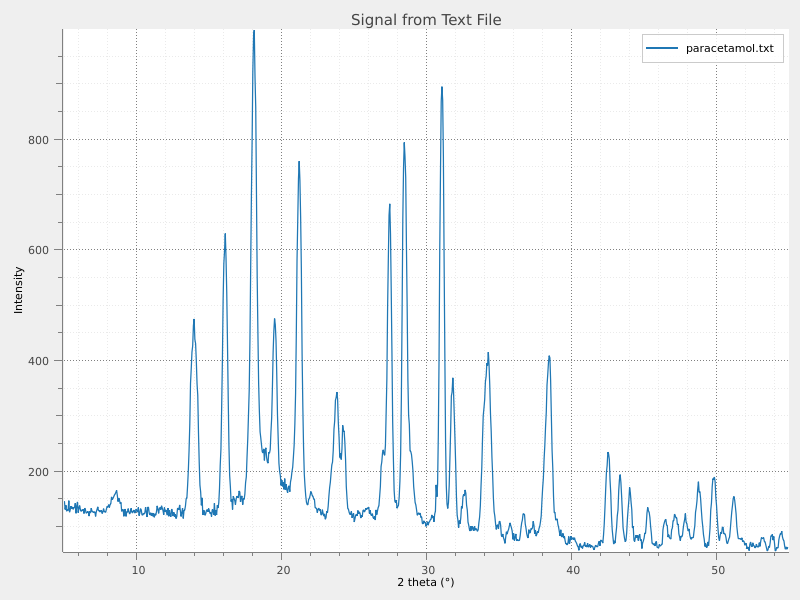
# Load a real spectrum from a text file
# This is a paracetamol (acetaminophen) UV-Vis absorption spectrum
filename = helpers.get_test_fnames("paracetamol.txt")[0]
signal_from_file = sigima.read_signal(filename)
# Visualize signal loaded from text file
viz.view_curves(signal_from_file, title="Signal from Text File")
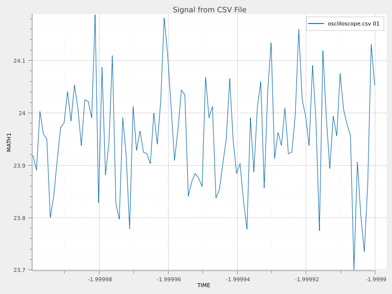
# Load another signal from a CSV file with multiple curves
csv_file = helpers.get_test_fnames("oscilloscope.csv")[0]
signals_from_csv = sigima.read_signals(csv_file)
# CSV files contain multiple signals; we'll show one
signal_from_csv = signals_from_csv[1]
# Visualize signal loaded from csv file
viz.view_curves(signal_from_csv, title="Signal from CSV File")
print("\n✓ Signals loaded from files")
print(f" - {signal_from_file.title}: {signal_from_file.y.shape[0]} points")
print(f" - {signal_from_csv.title}: {signal_from_csv.y.shape[0]} points")
✓ Signals loaded from files
  - paracetamol.txt: 999 points
  - oscilloscope.csv 01: 100 points
It is interesting to remark here that when importing data from files, Sigima automatically extracts and preserves metadata when possible. This includes:
Axis labels and units: Column headers from CSV files, variable names from MAT-Files, etc.
Acquisition parameters: DICOM headers, instrument settings, timestamps
Physical coordinates: Pixel spacing, origin coordinates when stored in the file
The extracted metadata is seamlessly integrated into the signal or image object, making it available for processing, analysis, and visualization without manual configuration.
{'CH6_D0': 0,
 'CH6_D1': 0,
 'CH6_D2': 0,
 'CH6_D3': 1,
 'CH6_D4': 1,
 'CH6_D5': 0,
 'CH6_D6': 0,
 'CH6_D7': 1,
 'source': '/home/docs/checkouts/readthedocs.org/user_builds/sigima/checkouts/stable/sigima/data/tests/curve_formats/oscilloscope.csv'}
Method 3: Creating signals from NumPy arrays#
When you already have data in NumPy arrays (from calculations, other libraries, or custom data sources), you can wrap them in Sigima signal objects to benefit from metadata handling and processing functions.
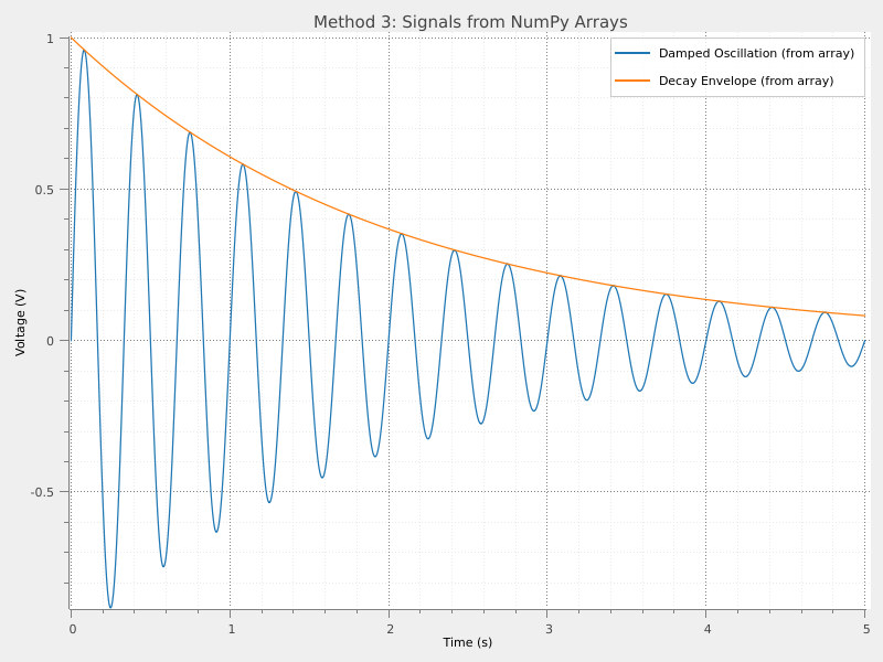
# Create custom data: a damped oscillation (e.g., RLC circuit response)
t = np.linspace(0, 5, 1000)
damping = np.exp(-0.5 * t)
oscillation = np.sin(2 * np.pi * 3 * t)
y_damped = damping * oscillation

signal_from_array = sigima.create_signal(
    title="Damped Oscillation (from array)",
    x=t,
    y=y_damped,
    units=("s", "V"),
    labels=("Time", "Voltage"),
)

# Create the envelope signal: upper and lower bounds of the oscillation
# This is useful for analyzing the decay rate and quality factor
y_envelope_upper = damping
y_envelope_lower = -damping

# We'll create a signal showing the upper envelope
signal_envelope = sigima.create_signal(
    title="Decay Envelope (from array)",
    x=t,
    y=y_envelope_upper,
    units=("s", "V"),
    labels=("Time", "Amplitude"),
)

print("\n✓ Signals created from NumPy arrays")
print(f"  - {signal_from_array.title}: {signal_from_array.y.shape[0]} points")
print(f"  - {signal_envelope.title}: {signal_envelope.y.shape[0]} points")

# Visualize signals created from NumPy arrays
viz.view_curves(
    [signal_from_array, signal_envelope],
    title="Method 3: Signals from NumPy Arrays",
    object_name="signals_from_arrays",
)
✓ Signals created from NumPy arrays
  - Damped Oscillation (from array): 1000 points
  - Decay Envelope (from array): 1000 points
Summary#
This example demonstrated the three main ways to create signals in Sigima:
Synthetic generation: Fast creation of standard mathematical functions and distributions using parameter classes. Perfect for testing and simulation.
File loading: Read data from various scientific and common file formats, with automatic format detection and metadata extraction. Essential for working with experimental data.
NumPy array conversion: Wrap existing array data with Sigima’s rich metadata and processing capabilities. Ideal for custom workflows and integration with other Python libraries.
All three methods produce equivalent Sigima objects that can be processed, analyzed, and visualized using the same set of tools and functions. Choose the method that best fits your workflow and data source.