
Note
Go to the end to download the full example code.
Fabry-Perot Interference Pattern#
This example demonstrates image processing techniques for analyzing Fabry-Perot interference patterns. It shows how to load experimental images, define regions of interest, detect circular contours, and extract intensity profiles for quantitative analysis of interference fringes.
- Usage:
python fabry_perot_example.py
The script demonstrates optical analysis workflows commonly used in interferometry, optical metrology, and precision measurements.
Importing necessary modules#
We start by importing all the required modules for image processing and visualization. To run this example, ensure you have all the required dependencies installed.
import sigima.enums
import sigima.objects
import sigima.proc.image
from sigima import viz
from sigima.tests.data import get_test_image
Load Fabry-Perot test images#
We load two sample image of Fabry-Perot interference patterns. These imags is included in the Sigima test data. We will analyze the interference fringes present in these images.
# Load the first Fabry-Perot test image
img1 = get_test_image("fabry-perot1.jpg")
print("✓ Successfully loaded fabry-perot1.jpg")
print(f"Image dimensions: {img1.data.shape}")
print(f"Data type: {img1.data.dtype}")
print(f"Intensity range: {img1.data.min()} - {img1.data.max()}")

# Visualize the original interference pattern
viz.view_images(img1, title="Fabry-Perot Interference Pattern #1")
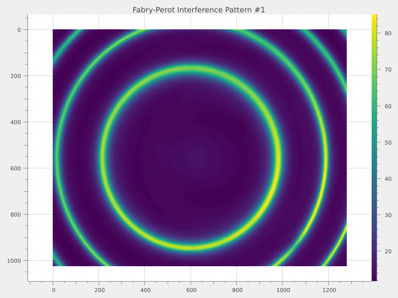
✓ Successfully loaded fabry-perot1.jpg
Image dimensions: (1024, 1280)
Data type: uint8
Intensity range: 7 - 94
Define circular ROI for fringe analysis#
We define a circular region of interest (ROI) centered on the image to focus our analysis on the central interference fringes.
# Calculate image center
center_x, center_y = 601, 559
roi_radius = 460  # Radius to capture the first few interference rings

print(f"\n✓ Image center: ({center_x}, {center_y})")
print(f"ROI radius: {roi_radius} pixels")
print("This ROI focuses analysis on the central interference pattern")

# Create circular ROI coordinates:
roi_coords = [center_x, center_y, roi_radius]

# Apply circular ROI to the image
img1.roi = sigima.objects.create_image_roi("circle", roi_coords, indices=True)

print("✓ Circular ROI applied to image")

# Visualize image with ROI
viz.view_images(img1, title="Fabry-Perot with Circular ROI")
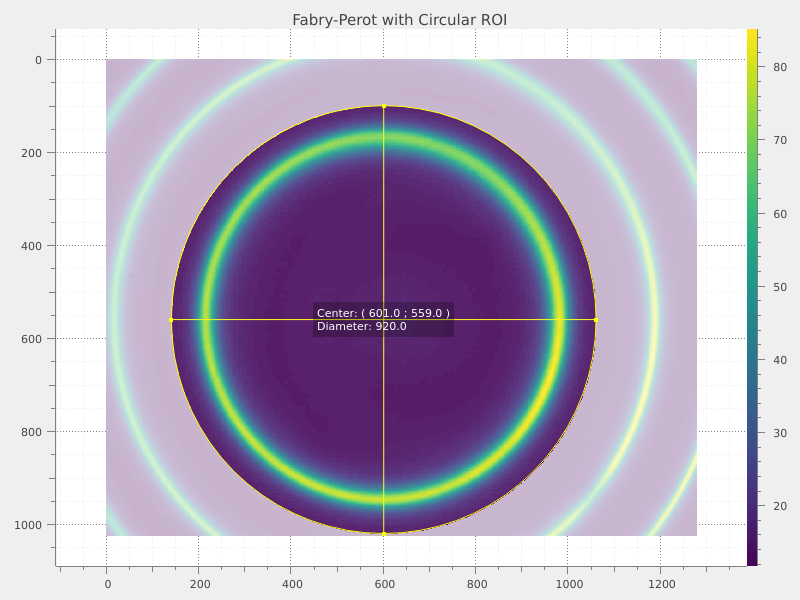
✓ Image center: (601, 559)
ROI radius: 460 pixels
This ROI focuses analysis on the central interference pattern
✓ Circular ROI applied to image
Configure contour detection for circular fringes#
We can now detect circular contours in the defined ROI. This will help us identify the interference rings. To perform this, the first step is to set up the contour detection parameter.
# Set up contour shape detection parameter for circles
contour_param = sigima.proc.image.ContourShapeParam()
contour_param.shape = sigima.enums.ContourShape.CIRCLE
contour_param.threshold = 0.5  # Threshold for fringe detection

print("\n✓ Contour detection configured:")
print(f"Shape: {contour_param.shape}")
print(f"Threshold: {contour_param.threshold}")
print("This will detect circular interference fringes")
✓ Contour detection configured:
Shape: Circle
Threshold: 0.5
This will detect circular interference fringes
We can now perform the contour detection on the image using the configured parameters.
contour_results = sigima.proc.image.contour_shape(img1, contour_param)

print("\n✓ Contour detection completed for first image")
✓ Contour detection completed for first image
We can now print the detected circular contours and their properties
print(f"Number of circular contours detected: {len(contour_results.coords)}")

contour_df = contour_results.to_dataframe()
print("\nDetected contours data frame:")
print(contour_df)
Number of circular contours detected: 2

Detected contours data frame:
   roi_index           x           y           r
0          0  599.143664  554.735897  403.219910
1          0  595.389606  556.166651  367.348831
Extract horizontal intensity profile#
We can extract an intensity profile along a horizontal line through the center of the image. This profile will show the intensity variations across the interference fringes. As before, we need to set up the line profile extraction parameter.
# Configure line profile extraction
profile_param = sigima.proc.image.LineProfileParam()
profile_param.direction = "horizontal"
profile_param.row = center_y  # Extract profile through image center

print("\n✓ Horizontal profile configured:")
print(f"Direction: {profile_param.direction}")
print(f"Row: {profile_param.row} (image center)")

# Extract intensity profile
profile_signal1 = sigima.proc.image.line_profile(img1, profile_param)

print(f"✓ Profile extracted: {len(profile_signal1.y)} data points")
print(f"Intensity range: {profile_signal1.y.min():.1f} - {profile_signal1.y.max():.1f}")

# Visualize the intensity profile
viz.view_curves(
    [profile_signal1],
    title="Horizontal Intensity Profile - Image 1",
    xlabel="Position (pixels)",
    ylabel="Intensity",
)
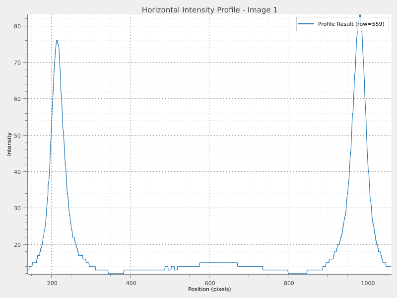
✓ Horizontal profile configured:
Direction: horizontal
Row: 559 (image center)
✓ Profile extracted: 919 data points
Intensity range: 12.0 - 83.0
Load the second Fabry-Perot image#
We want now to load the Analyze second Fabry-Perot image
try:
    # Load second test image
    img2 = get_test_image("fabry-perot2.jpg")
    print("\n✓ Successfully loaded fabry-perot2.jpg")
    print(f"Image dimensions: {img2.data.shape}")

    # Copy ROI settings from first image
    img2.metadata = img1.metadata  # This includes the ROI information

    # Visualize second image
    viz.view_images([img2], title="Fabry-Perot Interference Pattern #2")

except Exception as exc:
    raise RuntimeError("Failed to load second Fabry-Perot test image.") from exc
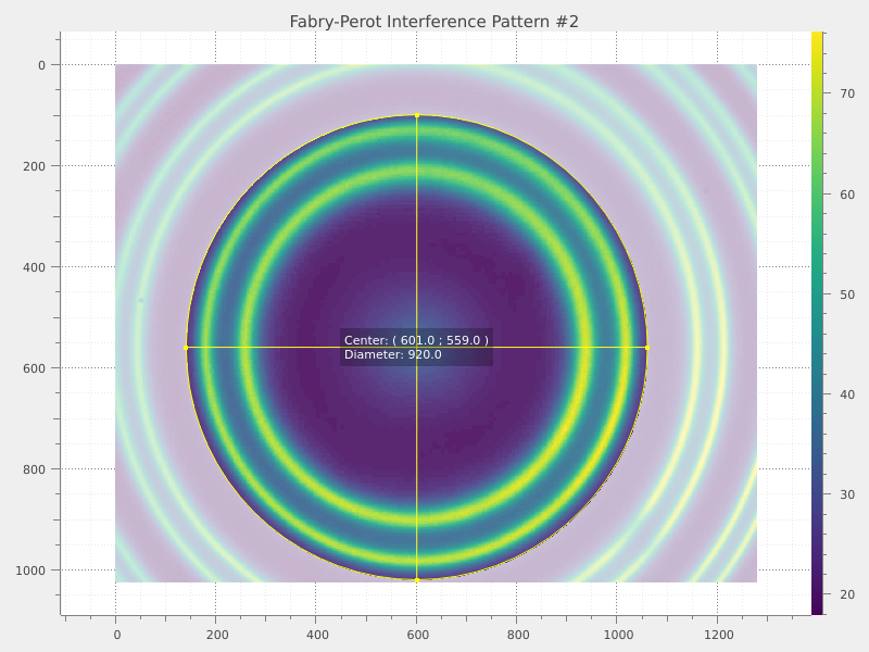
✓ Successfully loaded fabry-perot2.jpg
Image dimensions: (1024, 1280)
Contour detection on second image#
To perform the contour detection on the second image, we can reuse the same contour detection parameters defined earlier. This technique, applied to multiple images, allow to perform the same analysis on each of them and make comparisons easier.
# Apply the same contour detection to the second image
contour_results2 = sigima.proc.image.contour_shape(img2, contour_param)

print("✓ Contour detection completed for second image")

contour_df2 = contour_results2.to_dataframe()
print("\nDetected contours data frame (Image 2):")
print(contour_df2)
✓ Contour detection completed for second image

Detected contours data frame (Image 2):
   roi_index           x           y           r
0          0  599.872929  554.557532  437.578594
1          0  594.996655  555.561681  404.477426
2          0  599.469649  553.896986  363.131735
3          0  594.604309  555.225095  321.693888
Extract profile from second image and compare both profiles#
We can extract the horizontal intensity profile from the second image using the same profile extraction parameters defined earlier.
# Extract horizontal profile from second image
profile_signal2 = sigima.proc.image.line_profile(img2, profile_param)

print(f"\n✓ Profile extracted from second image: {len(profile_signal2.y)} points")
print(f"Intensity range: {profile_signal2.y.min():.1f} - {profile_signal2.y.max():.1f}")

# Compare profiles from both images
viz.view_curves(
    [profile_signal1, profile_signal2],
    title="Intensity Profile Comparison",
    xlabel="Position (pixels)",
    ylabel="Intensity",
)
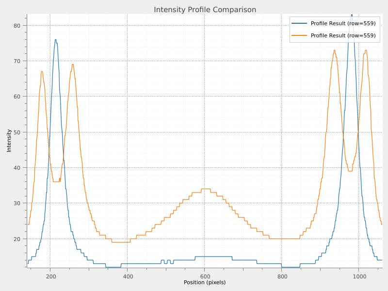
✓ Profile extracted from second image: 919 points
Intensity range: 19.0 - 73.0