
Note
Go to the end to download the full example code.
Laser Beam Size Measurement Example#
This example demonstrates comprehensive laser beam analysis techniques following the laser beam tutorial workflow. It shows how to load multiple laser beam images, analyze background noise with histograms, apply proper clipping, detect beam centroids, extract line and radial profiles, compute FWHM measurements, and track beam size evolution along the propagation axis.
The script demonstrates advanced optical beam characterization workflows commonly used in laser physics, beam quality assessment, and optical system design.
Importing necessary modules#
We start by importing all the required modules for image processing and visualization. To run this example, ensure you have all the required dependencies installed.
import numpy as np

import sigima.io
import sigima.objects
import sigima.params
import sigima.proc.image
import sigima.proc.signal
from sigima import viz
from sigima.tests import helpers
Load all laser beam images#
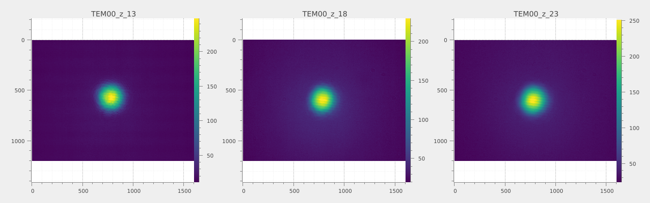
We load a series of laser beam images taken at different positions along the propagation axis (z-axis). The images are contained in the folder laser_beam and named following the pattern TEM00_z_*.jpg, where * is the z position in arbitrary units.
def load_laser_beam_images():
    """Load all laser beam test images from the test data directory.

    Returns:
        List of image objects loaded from TEM00_z_*.jpg files
    """
    # Get all TEM00 laser beam image files
    image_files = helpers.get_test_fnames("laser_beam/TEM00_z_*.jpg")

    # Sort files by z-position (extract number from filename)
    image_files.sort(key=lambda f: int(f.split("_z_")[1].split(".")[0]))

    # Load images
    images = []
    for filepath in image_files:
        img = sigima.io.read_image(filepath)
        # Extract z position from filename for proper naming
        z_pos = filepath.split("_z_")[1].split(".")[0]
        img.title = f"TEM00_z_{z_pos}"
        images.append(img)

    return images


images = load_laser_beam_images()

print(f"✓ Loaded {len(images)} laser beam images")
print("Image details:")
for i, img in enumerate(images):
    intensity_range = f"{img.data.min()}-{img.data.max()}"
    print(f"  {i + 1}. {img.title}: {img.data.shape}, range {intensity_range}")
✓ Loaded 14 laser beam images
Image details:
  1. TEM00_z_13: (1200, 1600), range 9-255
  2. TEM00_z_18: (1200, 1600), range 16-244
  3. TEM00_z_23: (1200, 1600), range 19-255
  4. TEM00_z_30: (1200, 1600), range 22-255
  5. TEM00_z_35: (1200, 1600), range 23-253
  6. TEM00_z_40: (1200, 1600), range 23-255
  7. TEM00_z_45: (1200, 1600), range 29-254
  8. TEM00_z_50: (1200, 1600), range 28-255
  9. TEM00_z_55: (1200, 1600), range 22-253
  10. TEM00_z_60: (1200, 1600), range 25-254
  11. TEM00_z_65: (1200, 1600), range 17-255
  12. TEM00_z_70: (1200, 1600), range 15-252
  13. TEM00_z_75: (1200, 1600), range 19-245
  14. TEM00_z_80: (1200, 1600), range 19-251
Visualize the first few images
print("\n✓ Visualizing sample images...")
viz.view_images_side_by_side(images[:3], title="Sample Laser Beam Images")
✓ Visualizing sample images...
Background noise analysis with histogram#
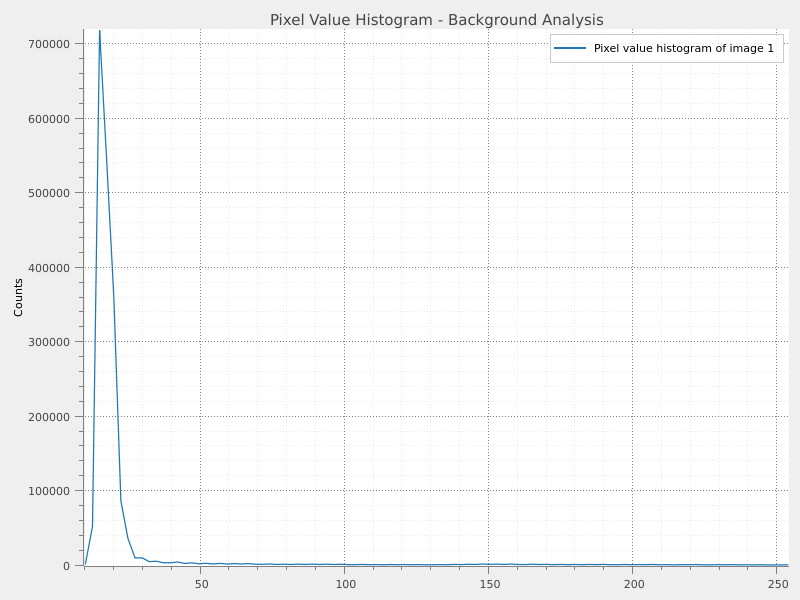
To analyze the background noise characteristics of the laser beam images, we create a histogram of pixel values from the first image. This helps us identify the noise floor and determine an appropriate clipping threshold.
print("\n--- Background Noise Analysis ---")

hist_param = sigima.params.HistogramParam()
hist_param.bins = 100
hist_param.range = (0, images[0].data.max())

hist = sigima.proc.image.histogram(images[0], hist_param)
hist.title = "Pixel value histogram of image 1"

print(f"✓ Generated histogram with {hist_param.bins} bins")
print(f"Histogram range: {hist_param.range[0]} - {hist_param.range[1]}")
print("The histogram shows background noise distribution")

# Visualize histogram
viz.view_curves([hist], title="Pixel Value Histogram - Background Analysis")
--- Background Noise Analysis ---
✓ Generated histogram with 100 bins
Histogram range: 0 - 255
The histogram shows background noise distribution
Based on the histogram analysis, we determine a clipping threshold around 30-35 LSB to effectively remove background noise from all images.
Background noise removal via clipping#
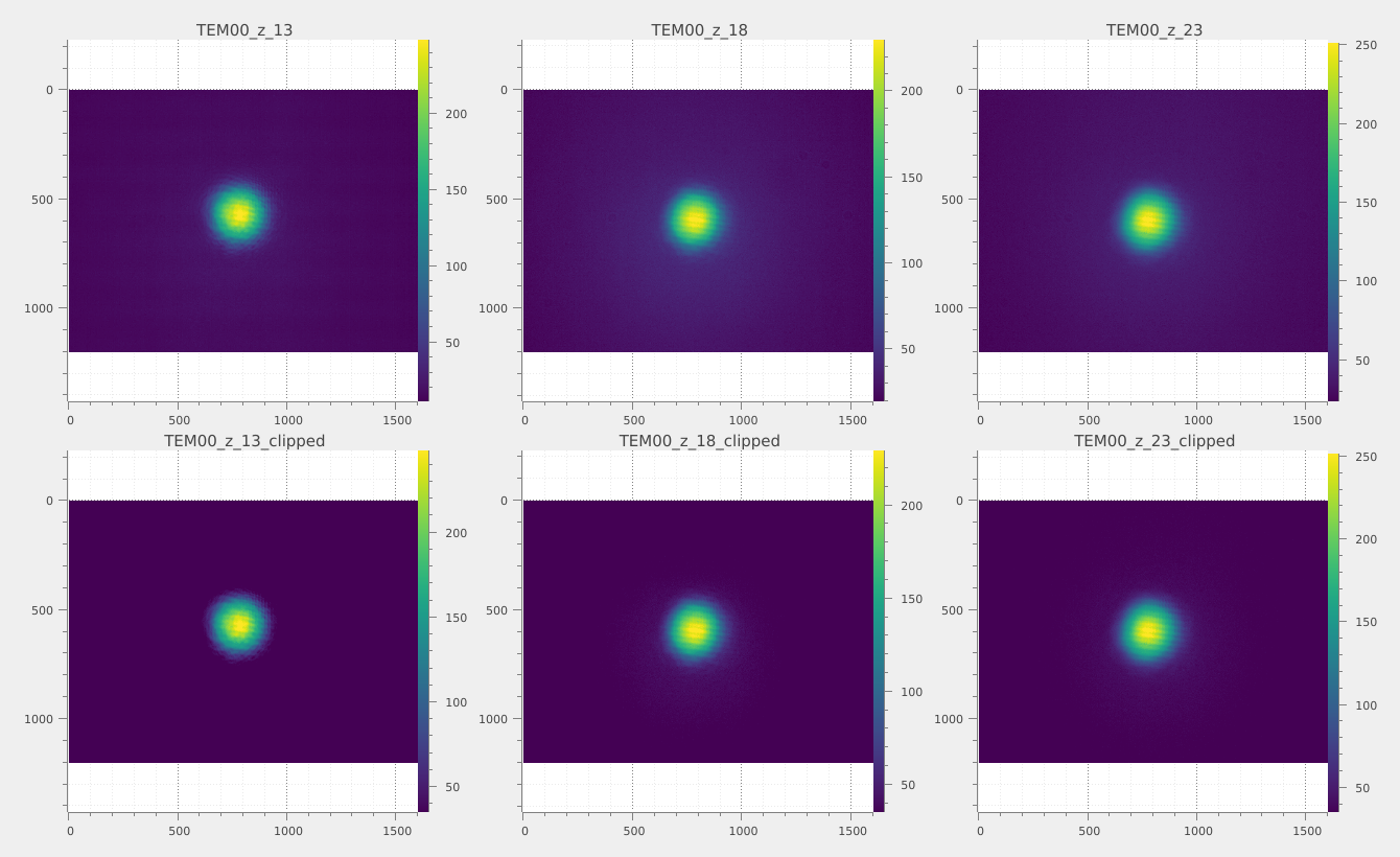
We set the threshold to 35 and we apply this clipping to each image in the dataset.
background_threshold = 35

print(f"Will use clipping threshold of {background_threshold} LSB")
Will use clipping threshold of 35 LSB
In order to perform the clipping, we create a ClipParam object and set the minimum value to the background threshold. We then apply the clipping to each image in the dataset.
print("\n--- Applying Background Clipping ---")
clip_param = sigima.params.ClipParam()
clip_param.lower = background_threshold  # Remove background noise below 35 LSB

clipped_images = []
for img in images:
    clipped_img = sigima.proc.image.clip(img, clip_param)
    clipped_img.title = f"{img.title}_clipped"
    clipped_images.append(clipped_img)

print(f"✓ Applied clipping of {clip_param.lower} LSB to all {len(images)} images")
print("Background noise below threshold has been removed")
--- Applying Background Clipping ---
✓ Applied clipping of 35.0 LSB to all 14 images
Background noise below threshold has been removed
We can now visualize some clipped images:
viz.view_images_side_by_side(
    images[:3] + clipped_images[:3],
    rows=2,
    title="Original and Clipped Images (First 3)",
)
Compute centroids for beam center detection#
Next, we compute the centroid of each clipped image to determine the beam center. This is important for accurate profile extraction and FWHM measurements.
print("\n--- Computing Beam Centroids ---")

centroids = []
for img in clipped_images:
    centroid_result = sigima.proc.image.centroid(img)
    centroids.append(centroid_result.value)  # (x, y)
    print(f"  ✓ {img.title}: centroid at {centroid_result.value}")

print(f"\n✓ Successfully detected {len(centroids)}/{len(images)} centroids")
--- Computing Beam Centroids ---
  ✓ TEM00_z_13_clipped: centroid at (778.5338326498419, 568.560005100494)
  ✓ TEM00_z_18_clipped: centroid at (785.7229313375627, 605.2159848744161)
  ✓ TEM00_z_23_clipped: centroid at (788.0762698963509, 605.6010279017113)
  ✓ TEM00_z_30_clipped: centroid at (795.3261027473541, 604.8806997507581)
  ✓ TEM00_z_35_clipped: centroid at (807.317154478579, 598.5952357707573)
  ✓ TEM00_z_40_clipped: centroid at (807.5259906509103, 600.6903181486724)
  ✓ TEM00_z_45_clipped: centroid at (818.739093714756, 594.1020243075966)
  ✓ TEM00_z_50_clipped: centroid at (815.9351210354206, 594.2577125051446)
  ✓ TEM00_z_55_clipped: centroid at (796.369697379878, 612.9430794831676)
  ✓ TEM00_z_60_clipped: centroid at (804.9800833526996, 632.2939961084006)
  ✓ TEM00_z_65_clipped: centroid at (787.5180304939635, 651.716668240321)
  ✓ TEM00_z_70_clipped: centroid at (786.8732160375479, 674.4876498869384)
  ✓ TEM00_z_75_clipped: centroid at (794.4038799919499, 655.1255080830181)
  ✓ TEM00_z_80_clipped: centroid at (794.5689506360085, 668.1613658534636)

✓ Successfully detected 14/14 centroids
Extract line profiles through beam centers#
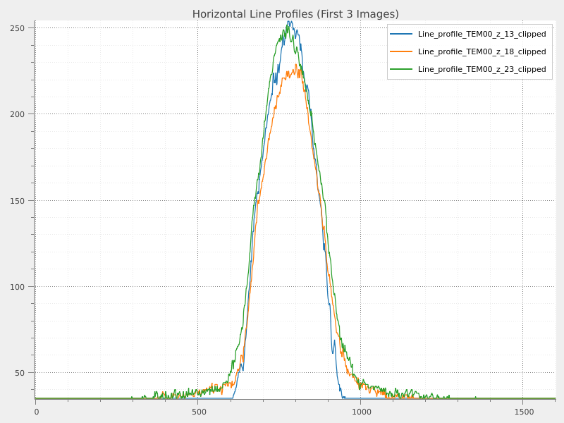
We extract horizontal line profiles through the detected centroids of each clipped image. This provides insight into the beam intensity distribution along a horizontal cross-section.
print("\n--- Extracting Line Profiles ---")

line_profiles = []
for i, (img, centroid_coords) in enumerate(zip(clipped_images, centroids)):
    # Create line profile parameters for horizontal line through centroid
    line_param = sigima.proc.image.LineProfileParam()
    line_param.direction = "horizontal"
    line_param.row = int(centroid_coords[1])  # Use centroid y-coordinate as row

    # Extract line profile
    profile = sigima.proc.image.line_profile(img, line_param)
    profile.title = f"Line_profile_{img.title}"
    line_profiles.append(profile)
    print(f"  ✓ Extracted line profile for {img.title} at row {line_param.row}")

print(f"\n✓ Generated {len(line_profiles)} line profiles")

# Visualize some line profiles
viz.view_curves(line_profiles[:3], title="Horizontal Line Profiles (First 3 Images)")
--- Extracting Line Profiles ---
  ✓ Extracted line profile for TEM00_z_13_clipped at row 568
  ✓ Extracted line profile for TEM00_z_18_clipped at row 605
  ✓ Extracted line profile for TEM00_z_23_clipped at row 605
  ✓ Extracted line profile for TEM00_z_30_clipped at row 604
  ✓ Extracted line profile for TEM00_z_35_clipped at row 598
  ✓ Extracted line profile for TEM00_z_40_clipped at row 600
  ✓ Extracted line profile for TEM00_z_45_clipped at row 594
  ✓ Extracted line profile for TEM00_z_50_clipped at row 594
  ✓ Extracted line profile for TEM00_z_55_clipped at row 612
  ✓ Extracted line profile for TEM00_z_60_clipped at row 632
  ✓ Extracted line profile for TEM00_z_65_clipped at row 651
  ✓ Extracted line profile for TEM00_z_70_clipped at row 674
  ✓ Extracted line profile for TEM00_z_75_clipped at row 655
  ✓ Extracted line profile for TEM00_z_80_clipped at row 668

✓ Generated 14 line profiles
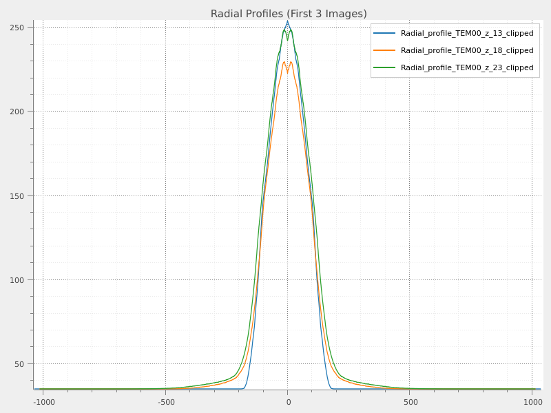
Extract radial profiles around beam centers#
We extract radial profiles centered on the detected centroids of each clipped image. This provides a circular intensity distribution useful for FWHM measurements.
print("\n--- Extracting Radial Profiles ---")

radial_profiles = []
for img in clipped_images:
    # Create radial profile parameters using automatic centroid detection
    radial_param = sigima.proc.image.RadialProfileParam()
    radial_param.center = "centroid"  # Use automatic centroid detection

    # Extract radial profile
    profile = sigima.proc.image.radial_profile(img, radial_param)
    profile.title = f"Radial_profile_{img.title}"
    radial_profiles.append(profile)
    print(f"  ✓ Extracted radial profile for {img.title}")

print(f"\n✓ Generated {len(radial_profiles)} radial profiles")
--- Extracting Radial Profiles ---
  ✓ Extracted radial profile for TEM00_z_13_clipped
  ✓ Extracted radial profile for TEM00_z_18_clipped
  ✓ Extracted radial profile for TEM00_z_23_clipped
  ✓ Extracted radial profile for TEM00_z_30_clipped
  ✓ Extracted radial profile for TEM00_z_35_clipped
  ✓ Extracted radial profile for TEM00_z_40_clipped
  ✓ Extracted radial profile for TEM00_z_45_clipped
  ✓ Extracted radial profile for TEM00_z_50_clipped
  ✓ Extracted radial profile for TEM00_z_55_clipped
  ✓ Extracted radial profile for TEM00_z_60_clipped
  ✓ Extracted radial profile for TEM00_z_65_clipped
  ✓ Extracted radial profile for TEM00_z_70_clipped
  ✓ Extracted radial profile for TEM00_z_75_clipped
  ✓ Extracted radial profile for TEM00_z_80_clipped

✓ Generated 14 radial profiles
We can now visualize some radial profiles
viz.view_curves(radial_profiles[:3], title="Radial Profiles (First 3 Images)")
Compute FWHM for radial profiles#
We compute the Full Width at Half Maximum (FWHM) for each radial profile to quantify the beam size. The FWHM is a standard metric for beam width.
print("\n--- Computing FWHM Measurements ---")

fwhm_vals = []
fwhm_param = sigima.params.FWHMParam()
fwhm_param.method = "zero-crossing"  # Standard FWHM method

for profile in radial_profiles:
    fwhm_result = sigima.proc.signal.fwhm(profile, fwhm_param)
    fwhm_vals.append(fwhm_result.value)
    print(f"  ✓ {profile.title}: FWHM = {fwhm_result.value:.2f} pixels")
--- Computing FWHM Measurements ---
  ✓ Radial_profile_TEM00_z_13_clipped: FWHM = 209.31 pixels
  ✓ Radial_profile_TEM00_z_18_clipped: FWHM = 213.12 pixels
  ✓ Radial_profile_TEM00_z_23_clipped: FWHM = 225.51 pixels
  ✓ Radial_profile_TEM00_z_30_clipped: FWHM = 237.13 pixels
  ✓ Radial_profile_TEM00_z_35_clipped: FWHM = 249.45 pixels
  ✓ Radial_profile_TEM00_z_40_clipped: FWHM = 263.25 pixels
  ✓ Radial_profile_TEM00_z_45_clipped: FWHM = 287.57 pixels
  ✓ Radial_profile_TEM00_z_50_clipped: FWHM = 298.89 pixels
  ✓ Radial_profile_TEM00_z_55_clipped: FWHM = 300.95 pixels
  ✓ Radial_profile_TEM00_z_60_clipped: FWHM = 321.70 pixels
  ✓ Radial_profile_TEM00_z_65_clipped: FWHM = 336.89 pixels
  ✓ Radial_profile_TEM00_z_70_clipped: FWHM = 349.77 pixels
  ✓ Radial_profile_TEM00_z_75_clipped: FWHM = 372.26 pixels
  ✓ Radial_profile_TEM00_z_80_clipped: FWHM = 388.66 pixels
That’s done, we can now print some FWHM statistics to check our results:
✓ FWHM Statistics:
  Valid measurements: 14/14
  Beam size range: 209.31 - 388.66 pixels
  Average beam size: 289.60 ± 56.83 pixels
Everything seems fine, we can now analyze the beam size evolution along the z-axis.
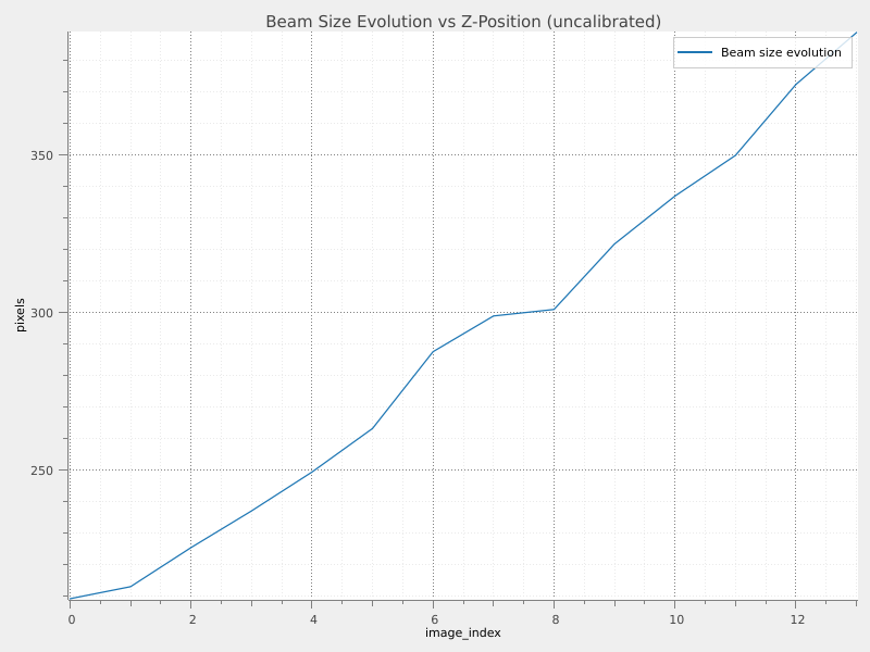
Analyze beam size evolution#
Having computed the FWHM for each radial profile, we can now analyze how the beam size evolves along the propagation axis (z-axis). This is useful to extract some meaningful information from all the numbers we have obtained. We create a signal representing the beam size evolution and visualize it.
print("\n--- Beam Size Evolution Analysis ---")

# Create a signal showing beam size evolution along z-axis
z_positions = list(range(len(fwhm_vals)))
beam_evolution = sigima.objects.create_signal(
    "Beam size evolution",
    np.array(z_positions),
    np.array(fwhm_vals),
    units=("image_index", "pixels"),
)

print(f"✓ Created beam evolution signal with {len(z_positions)} data points")

# Visualize beam size evolution
viz.view_curves(
    [beam_evolution], title="Beam Size Evolution vs Z-Position (uncalibrated)"
)
--- Beam Size Evolution Analysis ---
✓ Created beam evolution signal with 14 data points
The beam evolution signal currently uses image index as the x-axis, and even if we can see the trend, it is not very informative. It would be way better to have the x-axis in mm.
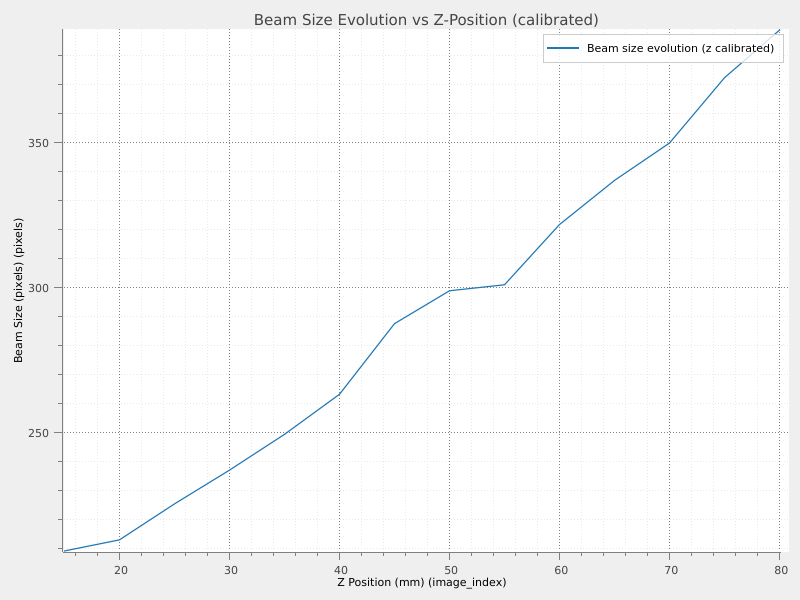
Apply z-axis calibration#
We apply a linear calibration to the x-axis of the beam evolution signal to convert image index to physical distance in mm. In Sigima there is the possibility to perform a linear axis calibration. We use the formula x’ = 5*x + 15, where x is the image index and x’ is the calibrated distance in mm.
print("\n--- Applying Z-Axis Calibration ---")

# Calibrate x-axis using the formula: x' = 5*x + 15 (convert to mm)
calib_param = sigima.proc.signal.XYCalibrateParam()
calib_param.axis = "x"
calib_param.a = 5.0  # Scale factor
calib_param.b = 15.0  # Offset

beam_evolution_calibrated = sigima.proc.signal.calibration(beam_evolution, calib_param)
beam_evolution_calibrated.title = f"{beam_evolution.title} (z calibrated)"

print(f"✓ Applied calibration: z' = {calib_param.a}*z + {calib_param.b}")
print("Z-axis now represents physical distance in mm")

# Visualize calibrated beam evolution
viz.view_curves(
    [beam_evolution_calibrated],
    title="Beam Size Evolution vs Z-Position (calibrated)",
    xlabel="Z Position (mm)",
    ylabel="Beam Size (pixels)",
)
--- Applying Z-Axis Calibration ---
✓ Applied calibration: z' = 5.0*z + 15.0
Z-axis now represents physical distance in mm