Spectrum Analysis

This example demonstrates advanced signal processing for spectroscopy analysis using a paracetamol spectrum. It shows how to apply noise reduction, region of interest selection, peak fitting, and detrending techniques available in Sigima. Each step builds upon the previous one to create a comprehensive analysis workflow.

Usage:

python paracetamol_example.py

The script demonstrates spectroscopy data processing workflows commonly used in analytical chemistry and materials science applications.

import numpy as np

import sigima.objects
import sigima.proc.signal
from sigima import viz
from sigima.tests.data import create_paracetamol_signal
from sigima.tools.signal import fitting, peakdetection

# Constants
XLABEL_ANGLE = "Angle"
YLABEL_INTENSITY = "Intensity"

Load test signal and initial visualization

We load a sample paracetamol spectrum included in the Sigima test data. This spectrum contains characteristic absorption peaks that we will analyze using various signal processing techniques.

# Load the paracetamol signal from test data
sig = create_paracetamol_signal()
x_orig, y_orig = sig.xydata

print("✓ Paracetamol spectrum loaded successfully!")
print(f"Signal contains {len(x_orig)} data points")
print(f"Energy range: {x_orig.min():.1f} to {x_orig.max():.1f} eV")
print(f"Intensity range: {y_orig.min():.1f} to {y_orig.max():.1f}")

# Visualize the original spectrum
viz.view_curves(sig, title="Paracetamol Spectrum - Original")

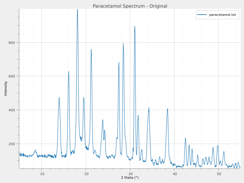
✓ Paracetamol spectrum loaded successfully!
Signal contains 999 data points
Energy range: 5.0 to 54.9 eV
Intensity range: 56.0 to 997.4

Apply Wiener filter for noise reduction

The signal is quite clean. Anyway, to illustrate the filtering capabilities of Sigima, we apply a Wiener filter to reduce any residual noise while preserving the spectral features.

sig_filt = sigima.proc.signal.wiener(sig)

print("\n✓ Wiener filter applied!")
print("The Wiener filter provides optimal noise reduction for signals")
print("with known statistical properties.")

# Compare original and filtered signals
viz.view_curves(
    [sig, sig_filt], title="Paracetamol Spectrum - Original vs Wiener Filtered"
)

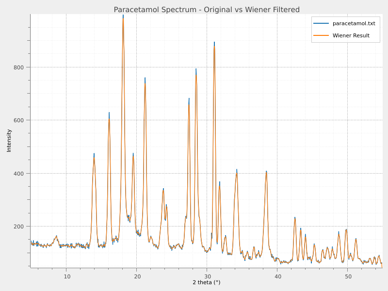
✓ Wiener filter applied!
The Wiener filter provides optimal noise reduction for signals
with known statistical properties.

Region of Interest (ROI) selection

We fistly focus our analysis on one of the peaks of interest. To to that, we define a region of interest (ROI) around the feature we want to analyze.

# Define ROI around the peak
roi_bounds = [35.5, 41.3]  # Energy range in eV
sig_filt.roi = sigima.objects.create_signal_roi(roi_bounds)

print(f"\n✓ ROI defined from {roi_bounds[0]} to {roi_bounds[1]} eV")
print("This focuses analysis on the primary absorption feature")

# Visualize the signal with ROI
viz.view_curves(sig_filt, title="Paracetamol Spectrum - Filtered with ROI")

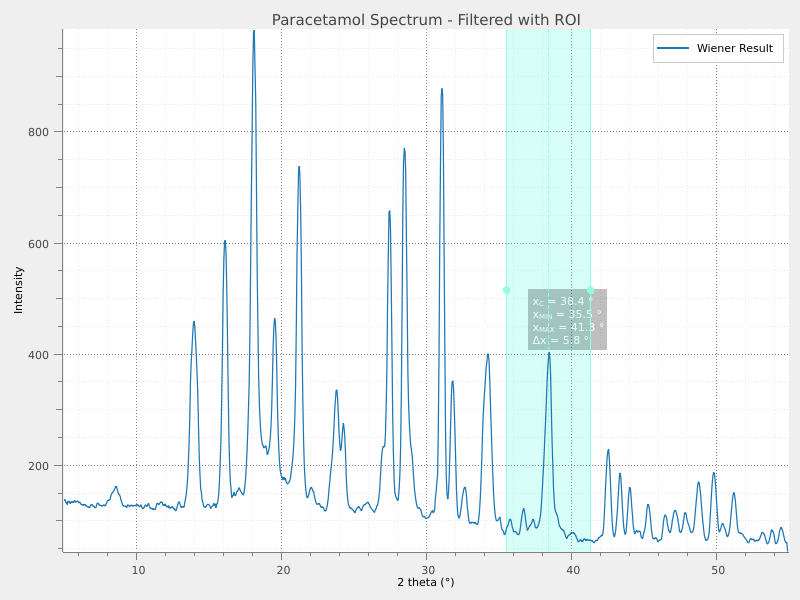
✓ ROI defined from 35.5 to 41.3 eV
This focuses analysis on the primary absorption feature

Gaussian fit on the peak

We can now fit the peak within the selected ROI using a Gaussian model. This provides quantitative parameters such as peak position, amplitude, and width.

# Perform Gaussian fit on the ROI-selected data
fit = sigima.proc.signal.gaussian_fit(sig_filt)

print("\n✓ Gaussian fit completed!")
print("This characterizes the main absorption peak with parameters:")
print("- Peak position (energy)")
print("- Peak amplitude (intensity)")
print("- Peak width (FWHM)")

# Visualize the signal with Gaussian fit
viz.view_curves([sig_filt, fit], title="Paracetamol Spectrum - ROI with Gaussian Fit")

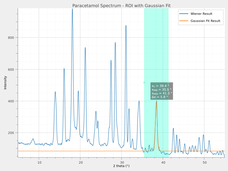
✓ Gaussian fit completed!
This characterizes the main absorption peak with parameters:
- Peak position (energy)
- Peak amplitude (intensity)
- Peak width (FWHM)

Linear detrending

After fitting the main peak, we may want to remove any baseline drift present in the entire spectrum.

The detrending function of Sigima performs a linear fit on the whole signal, including the peaks. In our signal peaks take a large part of the signal itself, witch is enough for signals where the peak are symmetrically distributed around the center, with more or less the same amplitude. This is not the case here, and we cannot expect this function to work well. It is however an interesting example to illustrate how Sigima functions can be combined to perform a more advanced analysis.

In order to visualize the limitation cited above, we apply the detrending function directly on the filtered signal. It’s important to remembre that we setted a ROI on the signal to focus the analysis on the main peak. We need to remove this ROI constraint to perform the detrending on the full signal.

# Remove ROI constraint for full signal detrending
sig_filt.roi = None

# Apply linear detrending to remove baseline drift
detrended_signal = sigima.proc.signal.detrending(sig_filt, method="linear")

print("\n✓ Linear detrending applied!")

# Compare filtered and detrended signals
viz.view_curves(
    [sig_filt, detrended_signal], title="Paracetamol Spectrum - Filtered vs Detrended"
)

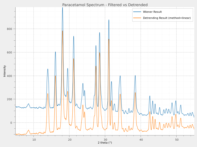
✓ Linear detrending applied!

The comparison shows, as expected, that the detrending function does not work well on this signal. This, as explained before, is due to the alogirithm used, which performs a linear fit on the whole signal, including the peaks. This effect is clearly visible on the plot: the peaks on the left, that are higher than the ones on the right, starts after the detrending at an intensity value lower than the ones on the right, and all peaks has a baseline under the zero.

Improved detrending with peak exclusion

An idea to overcome the limitation of the detrending function is suggested from the behavior of the detrended signal: we already identified the problem, which is that the linear fit is not performed on the baseline only, but also on the peaks.

To perform a better detrending, we can first thus detect the peaks and then perform a linear fit only on the non-peak regions. We reasonably expect this approach to provide a more accurate baseline estimation and a better detrended signal.

Automatic peak detection

We can use the peak detection function of Sigima to automatically identify the peaks in the spectrum. This function analyzes the signal and returns the indices of the detected peaks.

# Identify peaks in the detrended signal
peak_indices = peakdetection.peak_indices(sig_filt.y)

print("\n✓ Peak detection completed!")
print(f"Found {len(peak_indices)} potential peaks in the spectrum")

# Print detected peak positions
x_data = sig_filt.x
for i, peak_idx in enumerate(peak_indices):
    energy = x_data[peak_idx]
    intensity = sig_filt.y[peak_idx]
    print(f"  Peak {i + 1}: Energy = {energy:.2f} eV, Intensity = {intensity:.1f}")

✓ Peak detection completed!
Found 12 potential peaks in the spectrum
  Peak 1: Energy = 13.95 eV, Intensity = 459.0
  Peak 2: Energy = 16.10 eV, Intensity = 605.1
  Peak 3: Energy = 18.10 eV, Intensity = 983.5
  Peak 4: Energy = 19.50 eV, Intensity = 464.7
  Peak 5: Energy = 21.20 eV, Intensity = 738.3
  Peak 6: Energy = 23.80 eV, Intensity = 335.6
  Peak 7: Energy = 27.45 eV, Intensity = 658.2
  Peak 8: Energy = 28.45 eV, Intensity = 770.4
  Peak 9: Energy = 31.05 eV, Intensity = 878.3
  Peak 10: Energy = 31.80 eV, Intensity = 352.0
  Peak 11: Energy = 34.20 eV, Intensity = 400.5
  Peak 12: Energy = 38.45 eV, Intensity = 403.3

Multi-Gaussian fitting

We can now fit multiple Gaussian functions to the detected peaks. This allows us to characterize each peak individually and obtain parameters such as position, amplitude, and width for each peak.

# Perform multi-Gaussian fit using detected peaks
fitted_y, params = fitting.multigaussian_fit(
    sig_filt.x, sig_filt.y, peak_indices=peak_indices.tolist()
)

# Create fitted signal object for visualization
fitted_signal = sig_filt.copy()
fitted_signal.y = fitted_y
fitted_signal.title = "Multi-Gaussian Fit"

print("\n✓ Multi-Gaussian fitting completed!")
print("Each detected peak is fitted with individual Gaussian functions")

# Visualize the final fitting result
viz.view_curves(
    [sig_filt, fitted_signal],
    title="Paracetamol Spectrum - Detrended with Multi-Gaussian Fit",
)

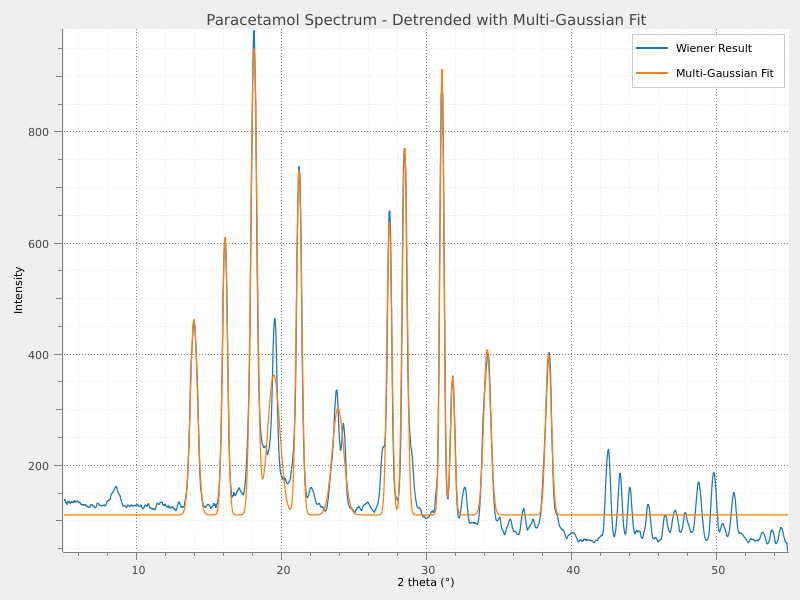
✓ Multi-Gaussian fitting completed!
Each detected peak is fitted with individual Gaussian functions

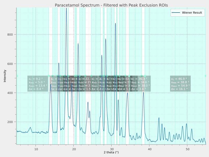
Defining ROI outside peaks for better detrending

To improve the detrending, we define ROIs that exclude the detected peaks. This allows us to fit the baseline only on the non-peak regions.

# Extract peak parameters from the multi-Gaussian fit
# Each peak has 3 parameters: amplitude, center, sigma
num_peaks = len(peak_indices)
peak_params = []

peaks_roi_bounds = np.zeros((num_peaks, 2))

for i in range(num_peaks):
    # Extract parameters for each Gaussian (amplitude, center, sigma)
    amplitude = params[f"amp_{i + 1}"]
    center = params[f"x0_{i + 1}"]
    sigma = params[f"sigma_{i + 1}"]
    peak_params.append([amplitude, center, sigma])

    # Define exclusion zone as center ± 2*sigma
    exclusion_start = center - 2 * abs(sigma)
    exclusion_end = center + 2 * abs(sigma)
    peaks_roi_bounds[i] = [exclusion_start, exclusion_end]

    print(f"Peak {i + 1}: Center = {center:.2f} eV, Sigma = {sigma:.3f}")
    print(f"  Exclusion zone: [{exclusion_start:.2f}, {exclusion_end:.2f}] eV")

# Create ROIs including detected peaks
roi = sigima.objects.create_signal_roi(peaks_roi_bounds)

# invert ROIs to exclude peaks
sig_filt.roi = roi.inverted(sig_filt.x.min(), sig_filt.x.max())

# Visualize the signal with new ROI
viz.view_curves(
    sig_filt, title="Paracetamol Spectrum - Filtered with Peak Exclusion ROIs"
)

Peak 1: Center = 13.94 eV, Sigma = 0.247
  Exclusion zone: [13.44, 14.43] eV
Peak 2: Center = 16.08 eV, Sigma = 0.177
  Exclusion zone: [15.72, 16.43] eV
Peak 3: Center = 18.08 eV, Sigma = 0.214
  Exclusion zone: [17.65, 18.50] eV
Peak 4: Center = 19.45 eV, Sigma = 0.423
  Exclusion zone: [18.60, 20.29] eV
Peak 5: Center = 21.19 eV, Sigma = 0.187
  Exclusion zone: [20.82, 21.56] eV
Peak 6: Center = 23.88 eV, Sigma = 0.394
  Exclusion zone: [23.09, 24.66] eV
Peak 7: Center = 27.42 eV, Sigma = 0.170
  Exclusion zone: [27.08, 27.76] eV
Peak 8: Center = 28.48 eV, Sigma = 0.173
  Exclusion zone: [28.14, 28.83] eV
Peak 9: Center = 31.05 eV, Sigma = 0.142
  Exclusion zone: [30.77, 31.33] eV
Peak 10: Center = 31.79 eV, Sigma = 0.146
  Exclusion zone: [31.50, 32.08] eV
Peak 11: Center = 34.17 eV, Sigma = 0.237
  Exclusion zone: [33.70, 34.65] eV
Peak 12: Center = 38.41 eV, Sigma = 0.201
  Exclusion zone: [38.00, 38.81] eV

We can now perform a linear fit on the signal using the defined ROIs to exclude the peaks. This will provide a more accurate baseline estimation.

fitted_signal = fit = sigima.proc.signal.linear_fit(sig_filt)

Finally, we can subtract the extended linear fit from the original filtered signal to obtain a better detrended signal. We can see that the baseline is now properly estimated, leading to a more accurate detrended signal.

better_detrended_signal = sigima.proc.signal.difference(sig_filt, fitted_signal)
better_detrended_signal.title = "Improved Detrended Signal"

print("\n✓ Improved detrending applied!")

# Compare filtered and better detrended signals
viz.view_curves(
    [sig_filt, better_detrended_signal],
    title="Paracetamol Spectrum - Filtered vs Improved Detrended",
    show_roi=False,
)

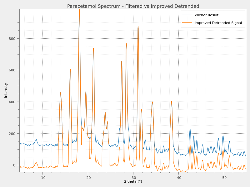
✓ Improved detrending applied!

To go futher…

In the last step we really improved the detrending of our signal. Anyway, several pics on the left of the signal are still not detected and the dentrending can be futher improved. We suggest you to experiment by tuning the parameters of the peak detection function and put your hands on the source code of this function to better understand how it works.